What Strategy is Best and How Do We Know?
A plethora of dispatching strategies have been suggested for maximizing a union’s total SP over the season, and new ideas are likely to emerge going forward. Perhaps the most well-known strategy is to maximize SP gained per dispatch (let’s call it Max Sp Per Train - MSPT; read more about this strategy in this post). A close relative of this strategy is to maximize the SP gained per unit of inventory. Another branch of strategies involves prioritizing certain jobs - for instance: storyline jobs, union-badged jobs, or perhaps the job that is closest to completion, and so on.
This ocean of ideas naturally begs the question: Which strategy is best?
Being the nerds that we are, we at BNG make use of Monte Carlo Simulation to compare the performance of different strategies. Monte Carlo Simulation, or MCS for short, is a numeric method that dates back to the Manhattan Project. Nicholas Metropolis, John von Neumann, and Stanislaw Ulam came up with the method to predict just how kablooey a nuclear bomb would be (not enough to usher in the end of the world by igniting the atmosphere forecasts suggested).
We won’t delve into the finer details of how kablooey-ness was calculated, but simply put, we simulate (more on that in another post) five or six sequences of union jobs, and then checks which strategy performs the best. We then simulate new sequences of jobs and check again which strategy performs the best. In every sequence, we have the same 25 players with exactly the same train fleet across each iteration of the simulation (their train fleets are different from each other though). After repeating the process a sufficient number of times, we can plot the statistical distribution of the season performance for each strategy. That way, we can see which strategy performed the best on average, how much risk each strategy entails (standard deviation) and the lower & upper level of performance.
As a very limited example, consider strategy Blue and Red. It doesn’t matter at this point what exactle these two strategies are. We have dozens of suggested strategies. These are merely two of them chosen haphazardly.
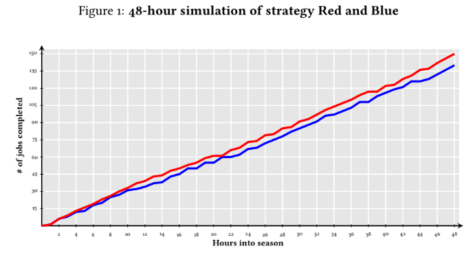
As shown by Figure 1, strategy Red seem to be better - the red line lies over the blue line more often than not. Furthermore, the vertical difference appears to be growing. Plotting the difference, the growing gap becomes more visible.

As discerned from Figure 2, there is considerable variation hour to hour, but there is a clear tendency. The trend in the time series can be estimated using what we call ordinary least squares (OLS) regression analysis. Let the difference between Red and Blue (Dif f RvB) be a function of the number of hours into the season (t).
In accordence with OLS, the slope coefficient (β1) can be calculated as the ratio be- tween the covariance of the dependent (Dif f Rvb) and independent variable (t), and the variance of the independent variable. Carrying out this calculation, we get a value of 0.1486. In other words, strategy Red tend to complete nearly 0.15 more jobs per hour. Extrapolating this trend, over a season, strategy Red will have completed 200 more jobs than strategy Blue (in this particular simulation, all jobs are side job - 500 SP per job).